How HEBBS Scores Memories, And Why Repeated Patterns Matter More
A deep dive into how HEBBS ranks, reinforces, and decays memories. Plus: why insights from larger clusters now score higher, and the cognitive science behind it.
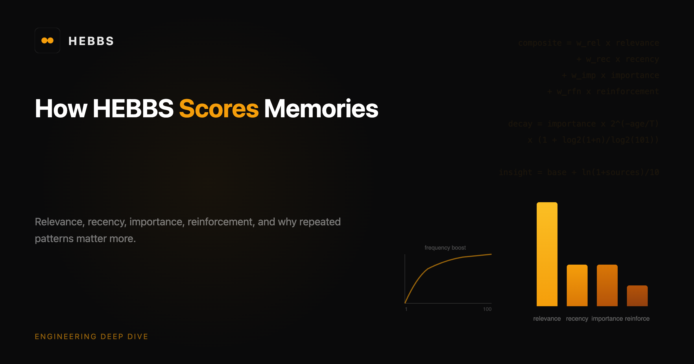
Every memory system faces the same question: when an agent asks “what do I know about this?”, which memories should surface first?
Vector databases answer with distance: the nearest embedding wins. That’s a start, but it ignores everything else. How important was this memory? How recently was it accessed? Has the agent relied on it before? And for insights derived from many observations, shouldn’t the breadth of evidence matter?
HEBBS answers all of these. This post explains the complete scoring system, from the moment a memory is created, through recall ranking, reinforcement, decay, and the new frequency-aware insight scoring.
The Four Signals
When you call recall(), HEBBS doesn’t just return the closest vectors. Every candidate memory is scored by four signals, weighted and combined into a single composite score:
composite_score = 0.5 x relevance
               + 0.2 x recency
               + 0.2 x importance
               + 0.1 x reinforcement
1. Relevance (50%)
This is the strategy-specific signal, the “how well does this memory match the query?” score. It varies by recall strategy:
- Similarity:
1.0 - L2_distancebetween query and memory embeddings - Temporal: Rank-based, where most recent memories get highest relevance
- Causal:
1.0 - (depth / max_depth), so closer causal connections score higher - Analogical: Blend of embedding similarity and structural relationship similarity
Relevance dominates at 50% weight because the retrieval strategy should be the primary signal. If you ask for similar memories, distance should matter most.
2. Recency (20%)
A linear decay from 1.0 to 0.0 over a configurable window (default: 30 days):
recency = max(0, 1.0 - age / max_age)A memory created 1 hour ago scores ~1.0. A memory from 15 days ago scores ~0.5. After 30 days, recency contributes nothing, but the memory can still rank high through other signals.
This is intentionally simple. Complex recency curves add tuning burden without clear benefit. Linear decay is predictable and easy to reason about.
3. Importance (20%)
Every memory has an importance score in [0.0, 1.0], set at creation time. For episode memories (raw observations), this comes from the caller. The agent or application decides what matters:
hebbs.remember("Customer mentioned they're evaluating competitors", importance=0.9)
hebbs.remember("Weather was nice during the call", importance=0.2)
Default importance is 0.5 if not specified. This value is immutable: once set, it doesn’t change. But as we’ll see, the effective importance changes over time through decay and reinforcement.
For insights (memories generated by the reflect pipeline), importance is computed differently. More on that below.
4. Reinforcement (10%)
Every time a memory is returned in a recall result, its access count increments. The reinforcement signal is logarithmic:
reinforcement = log2(1 + access_count) / log2(1 + cap)With the default cap of 100, this gives:
| Accesses | Reinforcement |
|---|---|
| 0 | 0.00 |
| 1 | 0.15 |
| 5 | 0.39 |
| 20 | 0.63 |
| 100 | 1.00 |
Logarithmic scaling means the first few accesses matter most. Going from 0 to 5 accesses is a bigger signal than going from 50 to 100. This matches how human memory works: the first few recalls of a fact consolidate it strongly, while additional repetitions have diminishing effect.
The 10% weight keeps reinforcement as a tiebreaker rather than a dominant signal. We don’t want a frequently-accessed but irrelevant memory to outrank a highly relevant one.
The Lifecycle: From Creation to Decay
Birth: remember()
When a memory is created:
importance = caller-provided or 0.5
decay_score = importance (starts equal)
access_count = 0
last_accessed_at = now
The memory enters the system at full strength. Its decay score equals its importance because no time has passed, so no decay has occurred.
Active Life: recall() + Reinforcement
Each time a memory appears in recall results, two things happen:
access_count += 1, strengthening the future reinforcement signallast_accessed_at = now, which resets the decay clock
That second point is critical. The decay formula uses last_accessed_at, not created_at, for its age calculation. A memory created 6 months ago but recalled yesterday is treated as 1 day old for decay purposes. Useful memories stay alive.
Background: Decay Sweeps
A background worker periodically recalculates every memory’s decay score:
decay_score = importance x 2^(-age / half_life) x reinforcement_multiplierWhere:
age = now - last_accessed_at(not created_at)half_life = 30 days(default)reinforcement_multiplier = 1 + log2(1 + access_count) / log2(1 + cap), range [1.0, ~2.0]
This creates a natural lifecycle:
- New memories start with decay_score equal to importance
- Accessed memories get their clock reset and reinforcement boosted, so they stay strong
- Neglected memories exponentially decay toward zero
- Memories below threshold (0.01) become auto-forget candidates
The half-life of 30 days means an unaccessed memory with importance 0.5 decays to 0.25 after a month, 0.125 after two months, and hits the auto-forget threshold around 6 months. But a single recall resets that clock entirely.
How Insights Are Scored Differently
Episode memories get their importance from the caller. But insights, memories generated by the reflect pipeline when it finds patterns across episodes, need a different approach. The caller didn’t create them. The system did.
The Reflect Pipeline
HEBBS periodically runs a four-stage reflect pipeline:
- Cluster: Group episode memories by embedding similarity
- Propose: LLM generates candidate insights per cluster (“these 15 customer calls all mention pricing confusion”)
- Validate: LLM validates candidates against source memories and existing insights
- Consolidate: Accepted insights are scored and stored
Insight Importance: Three Signals
An insight’s importance is computed from three signals:
importance = (0.7 x mean_source_importance + 0.3 x llm_confidence) + frequency_boostMean source importance (70% of base): The average importance of all episode memories that produced this insight. If the source memories were important, the insight should be too.
LLM confidence (30% of base): How confident the LLM is that this insight is valid, non-obvious, and useful. This is the qualitative judgment: “is this actually a meaningful pattern, or just noise?”
Frequency boost: ln(1 + source_count) / 10, a logarithmic boost based on how many source memories converged on this insight.
Why Frequency Matters
This is the newest addition to the scoring system, and it addresses a real gap.
Consider two insights generated by the reflect pipeline:
- Insight A: “Customers in the enterprise segment consistently ask about SSO integration”, derived from 30 call transcripts
- Insight B: “One customer mentioned preferring dark mode”, derived from 2 call transcripts
If both clusters happen to have similar average importance (say, 0.6) and the LLM gives both similar confidence (say, 0.8), the old formula would score them identically:
Old: 0.7 x 0.6 + 0.3 x 0.8 = 0.66 for bothBut Insight A is clearly more significant. It represents a pattern observed across 30 independent data points. Insight B is an anecdote from 2.
With frequency boost:
Insight A (30 sources): 0.66 + ln(31)/10 = 0.66 + 0.34 = 1.00
Insight B (2 sources):  0.66 + ln(3)/10  = 0.66 + 0.11 = 0.77
The logarithmic curve is important here. We want diminishing returns:
| Source Count | Frequency Boost |
|---|---|
| 1 | +0.07 |
| 3 | +0.14 |
| 10 | +0.24 |
| 20 | +0.31 |
| 50 | +0.39 |
| 100 | +0.46 |
Going from 3 to 10 sources adds +0.10. Going from 50 to 100 adds only +0.07. This prevents a single large cluster from completely dominating. 100 weak signals shouldn’t automatically outrank 10 strong ones.
The result is clamped to [0.0, 1.0], so the boost can elevate an insight’s importance but never beyond the maximum.
The Cognitive Science Parallel
This isn’t arbitrary engineering. It mirrors how human memory consolidation works.
In cognitive psychology, the frequency of co-occurrence is a primary driver of belief strength. If you hear the same claim from 20 independent sources, you hold it with more conviction than if you heard it once, even if each individual source is equally credible. This is the basis of the availability heuristic and illusory truth effect, but in a controlled, measurable form.
HEBBS makes this explicit and tunable. The logarithmic curve prevents the runaway effects that plague human cognition (where mere repetition creates false confidence). Instead, frequency is a bounded signal that contributes alongside source quality and LLM judgment.
Putting It All Together
Here’s the complete scoring flow for a memory’s lifetime:
CREATION (remember)
  Episode: importance = caller-provided (default 0.5)
  Insight: importance = 0.7 x mean_sources + 0.3 x llm_confidence + ln(1+count)/10

RECALL (query time)
  composite = 0.5 x relevance + 0.2 x recency + 0.2 x importance + 0.1 x reinforcement
  → Results sorted by composite score, top-k returned
  → Each returned memory: access_count++, last_accessed_at = now

DECAY (background sweeps, every hour)
  decay_score = importance x 2^(-age/half_life) x (1 + log2(1+accesses)/log2(101))
  → If decay_score < 0.01 → candidate for auto-forget
Three scoring systems, three different purposes:
- Importance is the memory’s intrinsic value, set once, never changes
- Composite score is the query-time ranking, changing with every query based on relevance, recency, and reinforcement
- Decay score is the long-term survival signal, changing over time based on age and usage
Together, they create a memory system where relevant memories surface first, useful memories stay alive, neglected memories fade, and insights backed by broad evidence rank above anecdotes.
That’s how memory should work.